Here are some Excel functions and tips, which might help you to format the data in your import file.
Gotcha’s to watch out for
Any leading zero’s will be lost when opening a csv type file. Eg, 0021 will revert to just 21. If that is a category number, then that will fine, as we have enough smarts to translate that when importing.
Price values like 204 and 204.00 are the same thing when importing into Tradevine.
Excel will convert large numbers like barcodes into scientific notation. Eg. 1234567890123 gets converted to 1.23457E+12. The workaround is to either open the file in a simple text editor like Notepad etc or deslect the barcode field when you import the file back into Tradevine.
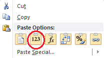
When copying and pasting the cell data created by a formula, make sure you paste the data as a value, not a formula. In later versions of Excel, right clicking where you are pasting into, will offer a 123 paste values option.

Handy hints
You can copy the formula in the top cell of a column quickly down to the bottom by mousing over the bottom right corner of the cell with the formula and when you see the bold plus symbol, double click it. It should automatically copy the data down to the last row unless your column has a mix of empty cells and non-empty cells.
Formatting your pricing type data
In most of these examples, we take a number from cell A2 and convert the format of the number.
Cell A2 = 123.45
| Mission | Formula | Outcome |
| Add a 65% markup | =A2*1.65 | 203.6925 |
| Round to 2 decimal places | =ROUND(A2*1.65,2) | 203.69 |
| Round up to the nearest whole dollar | =ROUNDUP(A2*1.65,0) | 204 |
| Round down to the nearest whole dollar | =ROUNDDOWN(A2*1.65,0) | 203 |
| Substitute the cents for 95c in the dollar | =TEXT(A2*1.65,"0.95") | 204.95 NB: this has rounded the dollar value and then applied the 95c |
| Substitute the cents for 95c in the dollar, but first round down to the nearest whole dollar | =TEXT(ROUNDDOWN(A2*1.65,0),"0.95") | 203.95 |
Formatting your text data
In these examples, we will build up some text using other text.
Cell A2 contains the word Gizmo. Cell B2 contains the value 123.45
| Mission | Build up some text from 4 different components |
| Formula | =CONCATENATE("This is the best ",A2," on the planet at just $",B2) |
| Outcome | This is the best Gizmo on the planet at just $123.45 |
| Mission | Build up some text, but format some of it onto a new line using CHAR(10) |
| Formula | =CONCATENATE("Model S-01725",CHAR(10),"This is the best ",A2," on the planet at just $",B2) |
| Outcome | Model S-01725 This is the best Gizmo on the planet at just $123.45 |
| Mission | Create some text to display over a few lines in a web page using HTML |
| Formula | =CONCATENATE(“S1416-“,A2,”<p>The one and only <b>Gizmo</b>.</p><p>Rated as the best around by the world’s most renown <i>obsessive compulsive</i> product buyers.</p> “) |
| Outcome | S1416-GIZMO The one and only Gizmo. Rated as the best around by the world’s most renown obsessive compulsive product buyers. |
| Mission | Replace the copyright symbol with HTML entity formatted text. Here our cell A3 contains the text: Protected by © 2013 |
| Formula | =REPLACE(A3,SEARCH("©",A3),1,"©") Here the Search function is looking for the position of the copyright symbol. The Replace function then only replaces that one character with our new HTML entity text of © |
| Outcome | Protected by © 2013 |
Common symbols
Always wanted to know how to insert those special symbols, like the symbol for copyright? These can be created by holding down the ALT key and punching in a three or four long sequence of numbers.
NB: if you intend to use these symbols and import the data, then you will need to save your import file in UTF-8 format. Alternatively, if the HTML Entity text exists for a symbol, then you can use this in your import file to create the symbol.
| Name | Example | Key Combination | HTML Entity |
| Bullet point | • | ALT + 0149 | • |
| Degrees | 45° or 17°C | ALT + 248 | ø |
| Diameter | Ø | ALT + 0216 | Ø |
| Copyright | © | ALT + 0169 | © |
| Registered | ® | ALT + 0174 | ® |
| Trademark | ™ | ALT + 0153 | ™ |
| Quarter | ¼ | ALT + 172 | ¼ |
| Half | ½ | ALT + 171 | ½ |
| Three Quarters | ¾ | ALT + 0190 | ¾ |
| Infinity | ∞ | ∞ | |
| Cents | ¢ | ALT + 0162 | ¢ |
| Micro | µ | ALT + 0181 | µ |
Tips
Here are some general Excel tips, which you may find useful.
To quickly enter a date use the keyboard shortcut CTRL with a semicolon ( CTRL + ; )
To enter the current time use the keyboard shortcut CTRL with SHIFT and a semicolon ( CTRL + SHIFT + ; )
To automatically size the width of all your columns, select the gap in the top left corner (above row 1 and left of column A), this should highlight the entire spreadsheet. Then double click the gap between any two column headers.

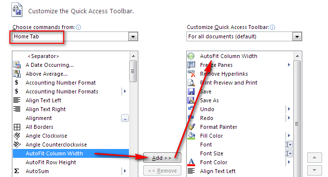
Alternatively, if you are a fan of customising your Quick Access Toolbar, then you can add the AutoFit Column Width command to your toolbar.

Again, you will need to select that top left space and then you can select the green AutoFit Column Width icon to auto size all the columns.
There is also an AutoFit Row Height if that appeals.